Adaptive Bandwidth
[2]:
import numpy as np

from jax import numpy as jnp
from jax import random

import matplotlib.pyplot as plt
import matplotlib.colors as mcolors

import sgGWR
An NVIDIA GPU may be present on this machine, but a CUDA-enabled jaxlib is not installed. Falling back to cpu.
[8]:
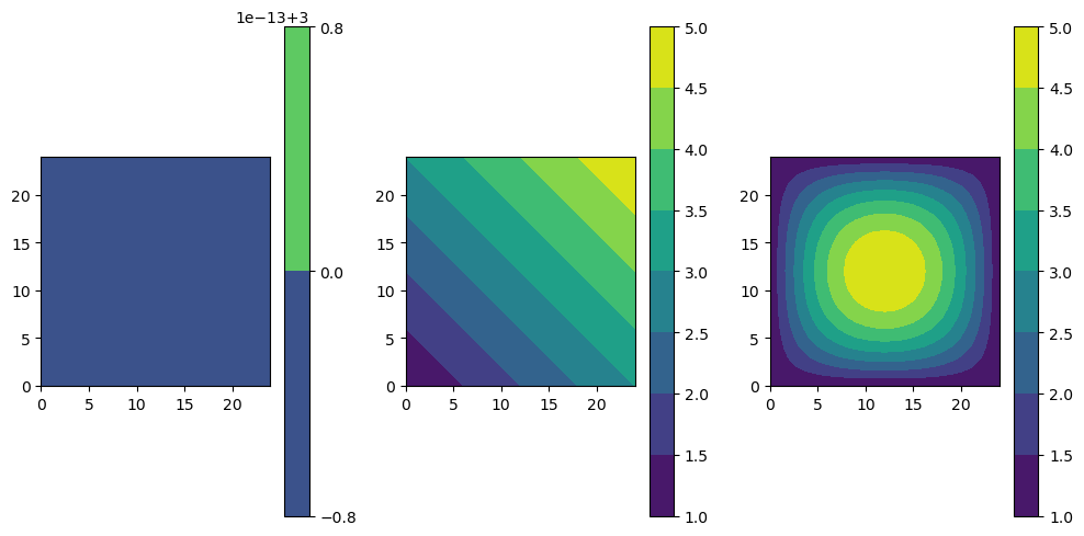
# spatial coefficient from
# Fotheringham, A. S., Yang, W., & Kang, W. (2017). Multiscale Geographically Weighted Regression (MGWR).
# Annals of the American Association of Geographers, 107(6), 1247–1265. https://doi.org/10.1080/24694452.2017.1352480

u0, v0 = jnp.arange(25), jnp.arange(25)
u, v = jnp.meshgrid(u0, v0)
u, v = u.flatten(), v.flatten()
N = len(u)
rngkey = random.PRNGKey(123)

beta = jnp.stack(
    [
        3 * jnp.ones(N),
        1 + (u + v) / 12,
        1 + (36 - jnp.square(6 - u / 2)) * (36 - jnp.square(6 - v / 2)) / 324,
    ]
).T
X = jnp.concatenate([jnp.ones((N, 1)), random.normal(rngkey, shape=(N, 2))], axis=1)
y = jnp.sum(X * beta, axis=1) + 0.5 * random.normal(rngkey, shape=(N,))
# %%
fig, axes = plt.subplots(1, 3, subplot_kw={"aspect": "equal"}, figsize=(10, 5))

for d in range(3):
    # cnorm = mcolors.Normalize(vmin=beta[:, d].min()-0.1, vmax=beta[:, d].max()+0.1)
    ct = axes[d].contourf(u0, v0, beta[:, d].reshape(len(u0), len(v0)))
    fig.colorbar(ct, ax=axes[d])

fig.tight_layout()
plt.show()
[5]:
sites = jnp.stack([u, v]).T

kernel = sgGWR.kernels.AdaptiveKernel(params=[10])
model_gwr = sgGWR.models.GWR(y, X, sites, kernel=kernel)

optim = sgGWR.optimizers.golden_section()
optim.run(model_gwr)

model_gwr.set_betas_inner()
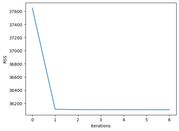
[6]:
sites = jnp.stack([u, v]).T

kernel = sgGWR.kernels.AdaptiveKernel(params=[10])
model_mgwr = sgGWR.models.MGWR(y, X, sites, kernel=kernel, base_class=sgGWR.models.GWR)

optims = [sgGWR.optimizers.golden_section()] * 3

model_mgwr.backfitting(optimizers=optims, run_params={"verbose": False})

plt.plot(model_mgwr.RSS)
plt.xlabel("iterations")
plt.ylabel("RSS")
plt.show()
[7]:
print("GWR bandwidth  = ", model_gwr.kernel.params[0])
print("MGWR bandwidth = ", [int(k.params[0]) for k in model_mgwr.kernel])
GWR bandwidth  =  29
MGWR bandwidth =  [161, 35, 26]
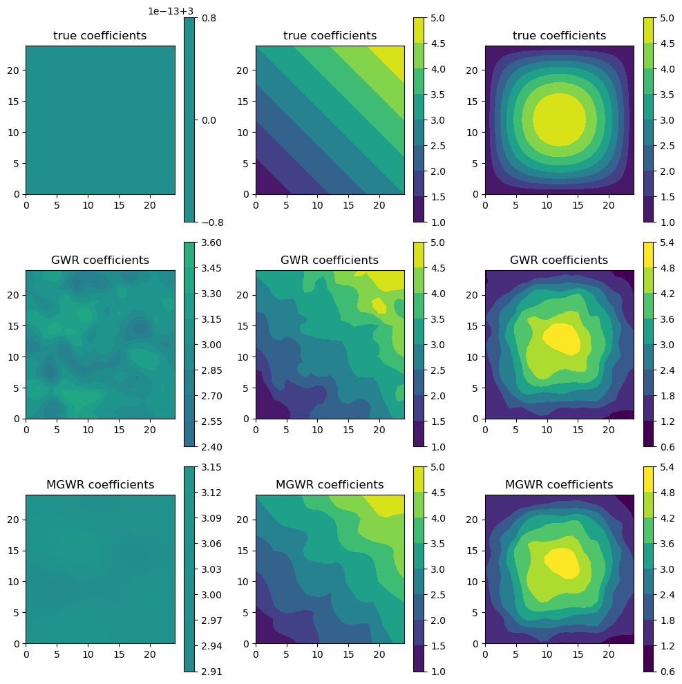
[15]:
fig, axes = plt.subplots(3, 3, subplot_kw={"aspect": "equal"}, figsize=(10, 10))

vmin, vmax = 1.0, 5.5
for d in range(3):
    axes[0][d].set_title("true coefficients")

    cnorm = mcolors.Normalize(vmin=vmin, vmax=vmax)#vmin=beta[:, d].min()-0.1, vmax=beta[:, d].max()+0.1)
    ct = axes[0][d].contourf(
        u0, v0, beta[:, d].reshape(len(u0), len(v0)), norm=cnorm,#vmin=1.0, vmax=5.0
    )
    cbar = fig.colorbar(ct, ax=axes[0][d])
    cbar.mappable.set_clim(vmin, vmax)

    axes[1][d].set_title("GWR coefficients")
    ct = axes[1][d].contourf(
        u0, v0, model_gwr.betas[:, d].reshape(len(u0), len(v0)), norm=cnorm,#vmin=1.0, vmax=5.0
    )
    cbar = fig.colorbar(ct, ax=axes[1][d])
    cbar.mappable.set_clim(vmin, vmax)

    axes[2][d].set_title("MGWR coefficients")
    ct = axes[2][d].contourf(
        u0, v0, model_mgwr.betas[:, d].reshape(len(u0), len(v0)), norm=cnorm,#vmin=1.0, vmax=5.0
    )
    cbar = fig.colorbar(ct, ax=axes[2][d])
    cbar.mappable.set_clim(vmin, vmax)

fig.tight_layout()
plt.show()
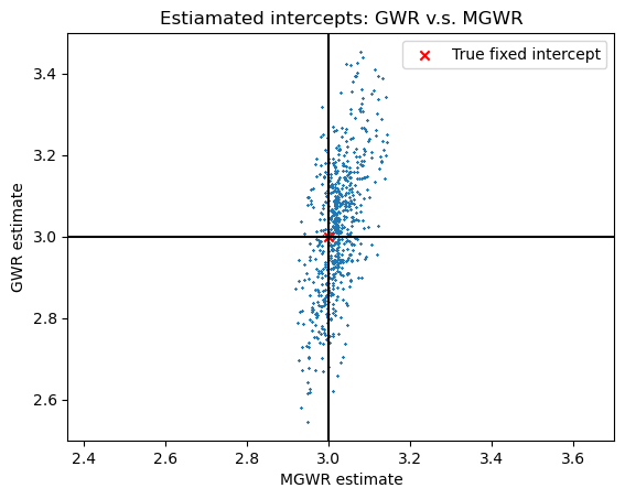
[16]:
plt.axis("equal")
plt.scatter(model_mgwr.betas[:, 0], model_gwr.betas[:, 0], s=1, marker="x")
plt.axvline(3, color="k")
plt.axhline(3, color="k")
plt.scatter(3, 3, marker="x", c="red", label="True fixed intercept")
plt.legend()
plt.title("Estiamated intercepts: GWR v.s. MGWR")
plt.xlabel("MGWR estimate")
plt.ylabel("GWR estimate")
plt.show()
[ ]:
[ ]: