How should we initialize the bandwidth parameter before tuning?

introduction

The initial value of bandwidth greatly affects the optimization efficency. If you choose ‘good’ initial value, you can save time to calibrate bandwidth. So, the initialization is important for practical use of GWR. Fortunately, you can easily employ the initialization heuristic proposed in Nishi & Asami (2024) with sgGWR.

import numpy as np
from scipy import interpolate

from jax import numpy as jnp
from jax import random

import matplotlib.pyplot as plt

import sgGWR

An NVIDIA GPU may be present on this machine, but a CUDA-enabled jaxlib is not installed. Falling back to cpu.

set up training data

First of all, we prepare the same simulation data to the tutorial Let’s start GWR bandwidth calibration with sgGWR!.

# This spatial coefficient model is inspired by Murakami et al. (2020)
def surface(sites, key, sigma, n_grid=30):
    s_min = jnp.min(sites, axis=0)
    s_max = jnp.max(sites, axis=0)

    x = jnp.linspace(s_min[0], s_max[0], num=n_grid)
    y = jnp.linspace(s_min[1], s_max[1], num=n_grid)
    x_ref, y_ref = np.meshgrid(x, y)
    x_ref = x_ref.flatten()
    y_ref = y_ref.flatten()
    ref = np.stack([x_ref, y_ref]).T

    d = np.linalg.norm(ref[:, None] - ref[None], axis=-1)
    G = jnp.exp(-d**2)

    beta_ref = random.multivariate_normal(key, mean=jnp.ones(len(ref)), cov=sigma**2*G, method="svd")

    interp = interpolate.RectBivariateSpline(x, y, beta_ref.reshape(n_grid, n_grid).T, s=0)
    beta = interp(sites[:,0], sites[:,1], grid=False)
    beta = jnp.array(beta)

    return beta

def DataGeneration(N, prngkey, sigma2=1.0):
    # sites
    key, prngkey = random.split(prngkey)
    sites = random.normal(key, shape=(N,2))

    # kernel
    G = jnp.linalg.norm(sites[:,None] - sites[None], axis=-1)
    G = jnp.exp(-jnp.square(G))

    # coefficients
    key, prngkey = random.split(prngkey)
    beta0 = surface(sites, key, sigma=0.5)
    # beta0 = random.multivariate_normal(key, mean=jnp.ones(N), cov=0.5**2 * G, method="svd")
    key, prngkey = random.split(prngkey)
    beta1 = surface(sites, key, sigma=2.0)
    # beta1 = random.multivariate_normal(key, mean=jnp.ones(N), cov=2.0**2 * G, method="svd")
    key, prngkey = random.split(prngkey)
    beta2 = surface(sites, key, sigma=0.5)
    # beta2 = random.multivariate_normal(key, mean=jnp.ones(N), cov=0.5**2 * G, method="svd")

    beta = jnp.stack([beta0, beta1, beta2]).T

    # X
    key, prngkey = random.split(prngkey)
    X = random.normal(key, shape=(N,2))
    X = jnp.concatenate([jnp.ones((N,1)), X], axis=1)

    # y
    y = beta0 + beta1 * X[:,1] + beta2 * X[:,2]
    key, prngkey = random.split(prngkey)
    y += sigma2**0.5 * random.normal(key, shape=(N,))

    return sites, y, X, beta

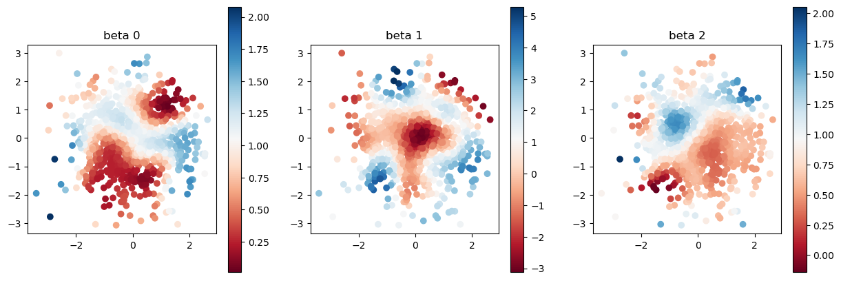
def plot_scatter(x, sites):
    fig = plt.figure(figsize=(15,5))
    for i in range(3):
        ax = fig.add_subplot(1,3,i+1)
        mappable = ax.scatter(sites[:,0], sites[:,1], c=x[:,i], cmap=plt.cm.RdBu)
        ax.set_title(f"beta {i}")
        ax.set_aspect("equal")
        fig.colorbar(mappable)
    # fig.show()

N = 1000
key = random.PRNGKey(123)
sites, y, X, beta = DataGeneration(N, key)
plot_scatter(beta, sites)

Bad initial value

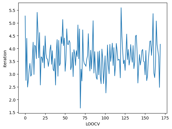
At first, let us check the performance when we select bad initial value. How this initial value affects the performance?

kernel = sgGWR.kernels.Exponential(params=[0.001]) # too small initial value
model = sgGWR.models.GWR(y=y, X=X, sites=sites, kernel=kernel)
optim = sgGWR.optimizers.SGDarmijo(learning_rate0=1.0)

loocv_loss = optim.run(model, maxiter=1000, batchsize=100)

print("calibrated bandwidth = ", model.kernel.params)

calibrated bandwidth =  [0.00118678]

plt.plot(loocv_loss)
plt.xlabel("LOOCV")
plt.ylabel("iteration")
plt.show()

Initialization with Heuristic

Next, we initialize bandwidth with kernel.init_params method. To use this method, you need to pass the coordinates of your dataset as sites argument.

You can also use idx argument to specify the index of sites which is referred to initialize. If idx=None, all data are refered. idx is useful when you handle very big data because if you refer all of your data in initialization step, you will spend long time. You don’t need to spend long time for initialization because the bandwidth parameter will be optimized later.

kernel2 = sgGWR.kernels.Exponential(params=[1.0])
kernel2.init_param(sites=sites, idx=None)
model2 = sgGWR.models.GWR(y=y, X=X, sites=sites, kernel=kernel2)
optim2 = sgGWR.optimizers.SGDarmijo(learning_rate0=1.0)

loocv_loss2 = optim2.run(model2, maxiter=1000, batchsize=100)

print("calibrated bandwidth = ", model2.kernel.params)

calibrated bandwidth =  [8.72599]

plt.plot(loocv_loss, label="bad initialization")
plt.plot(loocv_loss2, label="initialization with heuristics")
plt.xlabel("LOOCV")
plt.ylabel("iteration")
plt.legend()
plt.show()

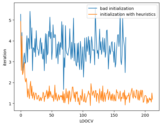
If you select bad initial value, it will cause to fail optimization and raise numerical errors. Our heuristic is to avoid such bad values automatically.

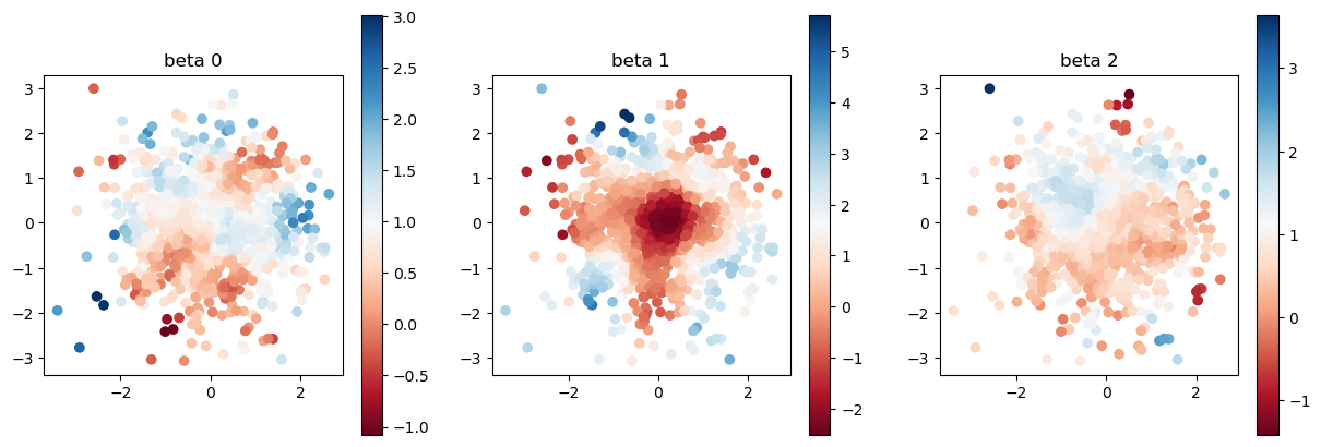
At the end of this tutorial, let us compare estimated coefficient. When the initial value is bad, the estimated coefficients are far from the true values.

model.set_betas_inner()

print("estimated coefficient with bad initial value")
plot_scatter(model.betas, sites)

estimated coefficient with bad initial value

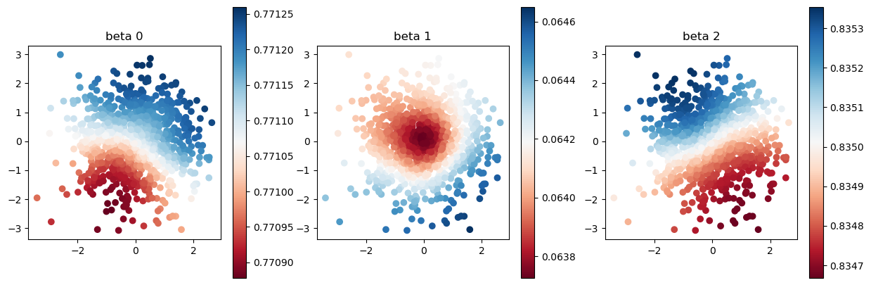
model2.set_betas_inner()

print("estimated coefficient with automatic initial value")
plot_scatter(model2.betas, sites)

estimated coefficient with automatic initial value

print("true coefficients")
plot_scatter(beta, sites)

true coefficients

Reference

• Hayato Nishi, & Yasushi Asami (2024). “Stochastic gradient geographical weighted regression (sgGWR): Scalable bandwidth optimization for geographically weighted regression”. International Journal of Geographical Information Science, Vol. 38, Issue: 2 pp.354-380, https://doi.org/10.1080/13658816.2023.2285471